PolicyLab

A few weeks ago, our team promised to share some of the ways in which we seek to validate our “COVID-Lab: Mapping COVID-19 in Your Community” models and improve them over time. So, we’re back with some details of our procedures and methodology for this validation work, which takes up considerable time weekly. 

Each week, we release our models’ four-week county-level case projections and reproduction numbers (Rs), or the estimate of how many additional individuals will get COVID-19 for every one person infected. These projections are based on anticipated social distancing levels and weather patterns for a given region. We estimate social distancing levels by holding constant the last week’s social distancing measurements and we use historical averages for temperature and humidity to formulate our weather estimates. We also assess our predictive accuracy weekly by running our models for the previous two weeks assuming the actual social distancing and temperature levels. This allows us to compare the observed case counts in a region with what our model predicted would happen. In general, these validation steps have revealed our predictions to be reasonably accurate over time.

The importance of these validation steps became especially important a few weeks ago when we were estimating that Maricopa County, Ariz. could exceed 20,000 cases daily and Miami might exceed 3,000 cases daily if they did not improve upon their degree of social distancing at the time. With these staggering numbers, we were compelled to delve further into the validation of our models to ensure that they would not extrapolate or otherwise produce inaccurate outlying projections under extreme conditions, resulting in over-estimation of projected cases in areas with dramatically surging case counts. 

This motivated us to consider whether adjustments to our foundational model might lead to better fits. The key factors in our foundational model include social distancing, weather, population density, and the recent trend or rate of growth in Rs. The foundational model also incorporates test positivity rates over time—which, as they grow, indicate potential infectious surge in the area, but when flat or declining would protect our models from overestimating risk that may be a result of increased testing capacity or contact tracing—and random effects for each county, which in simplistic terms means we allow the county to grow at a rate that it has established for itself over time. This protects our model from assuming, for example, that Pittsburgh would have the same epidemic curve as New York City, enabling the model to be adaptable to unmeasured local conditions in each county.

We explored adjusting this foundational model by adding or revising some of the key factors. For example:

• We tried adding random effects for a given metropolitan area, which would enable the model to learn across neighboring counties so it could capture phenomena like upticks in case counts within suburban collar counties spreading into city centers (which we’ve observed).
• We also recognized that our weather variables may have different effects in different climates, so we’ve explored introducing regional climate zones (e.g., the desert Southwest and the marine environments of the Pacific Northwest).
• We assessed various strategies for including the temperature effect, such as separating temperature and absolute humidity as separate factors and utilizing wet-bulb temperatures, which incorporate both temperature and humidity.
• Finally, we tried adding in absolute as well as relative test positivity rates for the previous week.

We’ve tested all of these variations on our original foundational model, using past data, to assess which result in the best estimates of future risk for most of our counties. 

This next part gets a little in the weeds, but we thought was important to share. Model validation must be done by training models on one subset of the data and testing their performance in another subset. In our validation process, we have used two different ways to select the training and testing subsets, either by counties or by time periods. Specifically, we have trained the models using a randomly selected 70% of counties and tested them on the other 30%. We have also trained the models using all of the counties included in our analysis between late March and May and tested them in the time period of June and July.

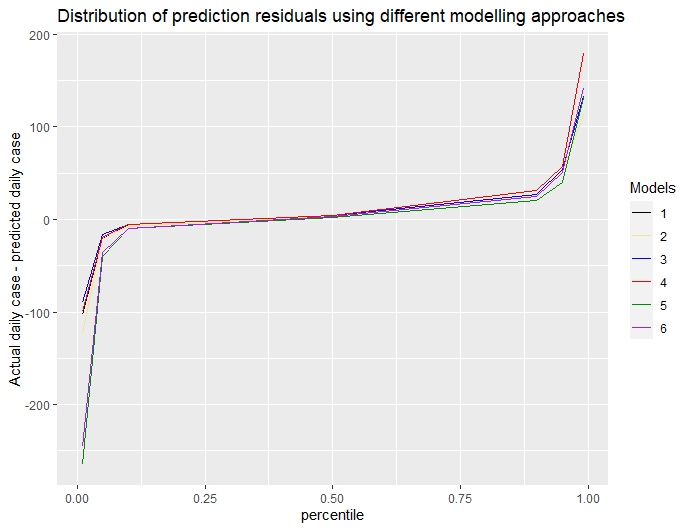
We consider two major measures to assess which model variation works best. First, we examine the “residuals,” or differences between actual and projected cases, from each model to choose the model that tends to have the smallest residuals across all of our counties. We plot that performance for the full set of counties and can quickly detect which of the models best reduces outliers and which ones were less accurate (see below). 

Second, we examine counties that have large residuals and compare the performance of different models for these “outlier” counties to understand the root causes of an inaccurate prediction. We also examine model performance in our outlier counties that have the highest case counts to see which models best approximated the rate of growth that was actually detected (see graphs for Maricopa, Harris and Miami-Dade Counties below).

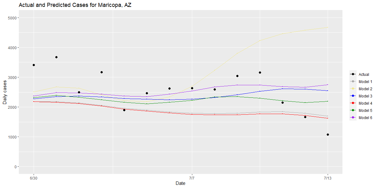
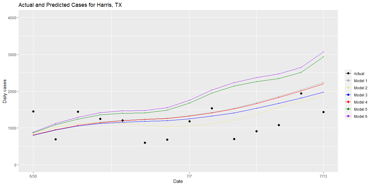
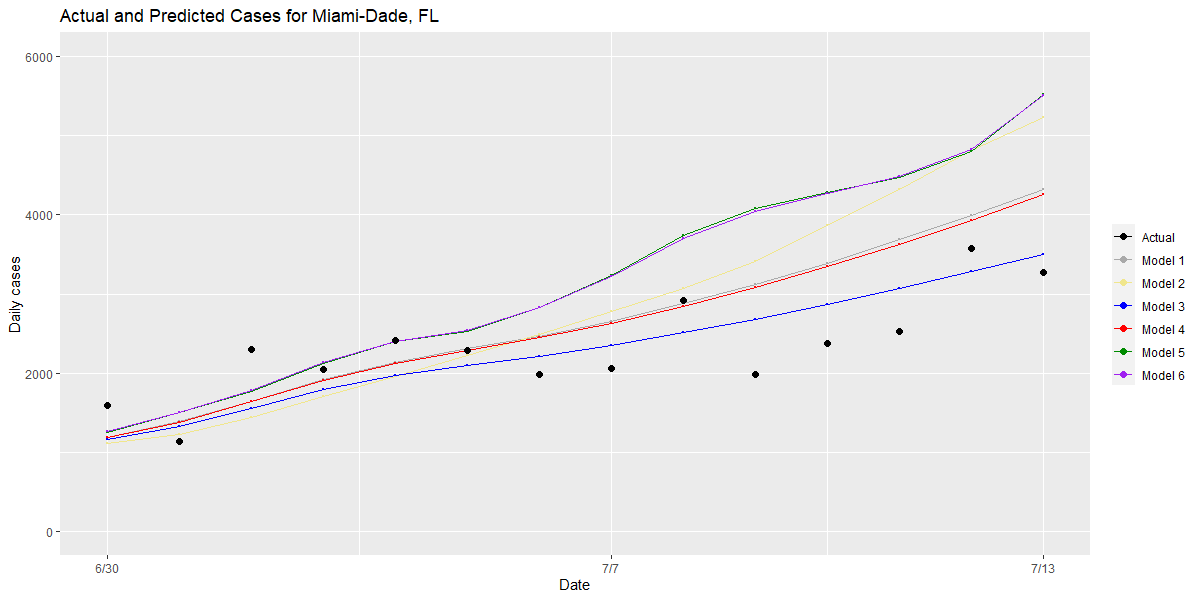
Bringing these two approaches together, this validation process has allowed us to make small, meaningful changes to our model over time, which we think provide the most robust and rigorous estimate of future risk within a county over the next one to four weeks. Those changes include:

• Returning to a model that includes wet-bulb temperatures rather than considering temperature and humidity as separate conditions,
• Adding a random effect for climate zones to our model, and
• Incorporating both the actual test positivity rate and the change in test positivity rate as a rolling average over the prior week.

Over time, we will continue to seek improvements our model, using these careful validation procedures to evaluate whether changes are beneficial, which will hopefully enable us to refine and adapt our model to the pandemic as it evolves and progresses.

Gregory Tasian, MD, MSc, MSCE, is an associate professor of urology and epidemiology and a senior scholar in the Center for Clinical Epidemiology and Biostatistics at the University of Pennsylvania Perelman School of Medicine. He is also an attending pediatric urologist in the Division of Urology at Children's Hospital of Philadelphia.